From Fractals to Functions: The Algorithmic Core of Machine Learning

A conceptual introduction into the learnable

How to connect fundamental complexity theory with machine learning? Well they all say the same thing. Image created with DALL-E.

Kolmogorov complexity is a fundamental concept from algorithmic information theory that measures the complexity of an individual object (such as a string or dataset) by the length of the shortest program that produces it. In machine learning theory, understanding the complexity of hypothesis classes and learning tasks is crucial for analyzing learnability. Notions like the Vapnik–Chervonenkis (VC) dimensionmeasure the capacity of function classes and appear in Probably Approximately Correct (PAC) learning theory. Interestingly, Kolmogorov complexity connects to these learning-theoretic concepts via Occam’s Razor and the minimum description length (MDL) principle — simpler (shorter) explanations tend to generalize better. This article provides an overview of Kolmogorov complexity (with equations and examples) and explores its connections to computability, PAC learnability, VC dimension, and recent developments in machine learning theory (such as PAC-Bayes analyses and the concept of Known Operator Learning). Throughout, we focus on the theoretical insights, illustrating key ideas with examples, code snippets, and references to recent research.

Kolmogorov Complexity: Definition and Key Properties

Kolmogorov complexity (KC), also known as algorithmic complexity or algorithmic entropy, of a finite object xxis defined as the length (in bits) of the shortest binary program (under a fixed universal Turing machine model) that produces x as output. Formally, if we fix a universal Turing machine U, the Kolmogorov complexity Kᵤ​(x) is:

where p ranges over programs that output x and ∣p∣ is the length of program p in bits. Intuitively, K(x) represents the smallest description length of x. For example, the string abababab... repeated 16 times has a short description (“print ab16 times”), whereas a comparably long string of random characters has no obvious shorter description than listing itself. Thus, the repetitive string has low Kolmogorov complexity, while a random-looking string has high Kolmogorov complexity.

Example — Compressible vs. Random Strings: To illustrate, consider two 32-character strings: one is abab... repeated 16 times, and the other is a 32-character random string:

import zlib 

pattern = "ab" * 16 
random_str = "4c1j5b2p0cv4w1x8rx2y39umgw5q85s7"
print("Pattern length:", len(pattern)) 
print("Compressed pattern length:", len(zlib.compress(pattern.encode()))) 
print("Random length:", len(random_str))
print("Compressed random length:", len(zlib.compress(random_str.encode())))

Running this yields:

Pattern length: 32  
Compressed pattern length: 12  
Random length: 32  
Compressed random length: 40

The patterned string compresses to 12 bytes (much smaller than its raw length of 32), whereas the random string actually grows slightly when compressed (40 bytes, due to compression overhead). This reflects that the patterned string has a short description (low complexity), while the random string is incompressible — essentially high Kolmogorov complexity. In general, regular structure in data allows significant compression, indicating lower Kolmogorov complexity, whereas random data is incompressible and has complexity roughly equal to its length.

Invariance and Uncomputability

A remarkable property of Kolmogorov complexity is that it is invariant up to an additive constant with respect to the choice of universal programming language or machine. That is, if Kᵤ​(x) and Kᵤ​’(x) are complexities defined using two different universal machines U and U′, their values differ by at most a constant independent of x. This makes the notion of KC well-defined for theoretical analysis. However, Kolmogorov complexity is uncomputable — there is no general algorithm that takes an object x and produces K(x) exactly. This is deeply related to Gödel’s and Turing’s seminal results: determining the shortest description can encode the halting problem. In fact, if one could compute Kolmogorov complexity, one could solve the halting problem and many other undecidable problems. As a consequence, we cannot write a program that outputs the exact K(x) for arbitrary x. We must instead rely on upper bounds (e.g. compressing data with practical algorithms gives an upper bound on Kolmogorov complexity) or use heuristic methods in practice. Despite this limitation, the concept of Kolmogorov complexity is extremely powerful for theoretical reasoning about information content and has strong links to probability and learning — for instance, via Solomonoff’s algorithmic probability, which assigns higher prior weight to simpler (shorter) hypotheses.

Kolmogorov Complexity and Occam’s Razor

The idea of preferring simpler explanations is formalized by Kolmogorov complexity: a simpler object has smaller K(x). This underpins the Occam’s Razor principle in a quantitative way. Indeed, Kolmogorov complexity can be viewed as an absolute version of model complexity, in contrast to classical measures like the number of parameters. In information-theoretic learning principles such as the Minimum Description Length (MDL) principle, one aims to minimize the sum of (1) the description length of the model/hypothesis and (2) the description length of the data given that model. MDL is essentially an application of Kolmogorov complexity ideas to statistical inference — selecting the hypothesis that gives the shortest overall encoding of data. While Kolmogorov complexity itself is not computable, practical MDL methods use computable proxy measures (like compression algorithms or parametric model coding schemes) to approximate this ideal.

An example of Kolmogorov complexity in action: the image above is a zoom of the Mandelbrot fractal “seahorse”. Storing it as raw pixels requires ~25 MB as gif, but a short program (using the fractal generation formula and coordinates) can reproduce it. Thus, the Kolmogorov complexity of this structured image is far less than 25 MB. In contrast, a truly random 25 MB image would have no shorter description than listing its pixels, so its Kolmogorov complexity would be ~25 MB.

PAC Learning and VC Dimension

In parallel to algorithmic complexity theory, Computational Learning Theory provides a framework for analyzing when a class of functions is learnable from data. Leslie Valiant’s Probably Approximately Correct (PAC) learning framework (1984) introduced rigorous definitions for learnability in terms of the ability of an algorithm to probably (with high probability 1−δ) find an approximately correct hypothesis (with error at most ε) using a feasible amount of data and computation. One of the central insights of PAC learning is that in order for a concept class (hypothesis space) to be learnable from finite data, the class must have limited complexity or capacity. Too rich a hypothesis space can shatter any dataset and lead to overfitting with no generalization guarantee.

VC Dimension

The Vapnik–Chervonenkis (VC) dimension is a classic measure of the capacity of a hypothesis class H. Informally, the VC dimension is the largest number of data points that H can label in all possible ways (i.e. the largest set of points that can be “shattered” by H). If a class has VC dimension d, it means there exist d points that the class can shatter (realize all 2dlabel configurations), but no set of d+1 points can be shattered.

A line has a VC dimension of 3. Image Source: baeldung.com

For example, the class of linear separators in the plane (R2) has VC dimension 3: one can find 3 non-collinear points that a line can shatter (separate in all 2^3=8 possible label assignments), but no 4 points in general position can be shattered by a single line. Intuitively, a line in 2D can classify any arrangement of 3 points (assign any point to positive/negative side appropriately), but with 4 points some labelings are impossible without a more complex (non-linear) boundary. In general, linear classifiers in Rd have VC dimension d+1 (including the bias term). Another example: the class of all binary classifiers on an infinite domain has infinite VC dimension — it can shatter arbitrarily large datasets (by simply memorizing labels), which implies it’s too rich to learn without further constraints.

PAC Learnability

A fundamental theorem in PAC learning states that a concept class H is PAC-learnable (with proper sample complexity bounds) if and only if H has finite VC dimension. When VC dimension is finite, we can quantify how many training samples are sufficient (and necessary) for learning. In particular, for a binary classification class with VC dimension d, to achieve error ≤ ε with probability ≥ 1−δ, on the order of

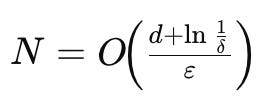
samples are needed. Likewise, any successful PAC learning algorithm for that class must use on the order of at least (d+ln(1/δ))/ε samples. For example, if d=3 and we desire 95% confidence (δ=0.05) and ε=0.1 error, the formula suggests needing on the order of (3+ln(20))/0.1≈60 samples. The key implication is that the number of samples required grows linearly with the complexity (VC dimension) of the hypothesis class. Thus, simpler hypothesis classes (smaller VC) generalize from less data, whereas extremely complex classes demand prohibitive amounts of data to avoid overfitting.

It’s worth noting that VC dimension is a combinatorial capacity measure and does not directly consider computational efficiency. There are classes with finite VC dimension that are information-theoretically learnable but for which no known polynomial-time learning algorithm exists (tying into computational complexity assumptions). PAC learning theory requires both polynomial sample complexity and polynomial-time algorithms for true feasibility. In practice, controlling the capacity of models (through network size, regularization, etc.) is crucial to ensure learnability, reflecting the same intuition captured by VC dimension and Occam’s razor in theory.

Occam’s Razor in Learning: From VC to Kolmogorov

VC dimension provides a way to quantify model complexity in terms of shattering ability, but Occam’s Razor hints at a more general principle: if a hypothesis h explains the data with a short description, it is likely to generalize well. In PAC theory, one can formalize Occam’s Razor via bounds that depend on the description length of the hypothesis. For instance, suppose a learning algorithm returns a hypothesis h that perfectly fits the training data and has description length ℓ bits (for example, ℓ=log2​∣H∣ if we identify the hypothesis within a finite class, or ℓ could be the length of the hypothesis encoded in some language). Then a version of Occam’s bound says that with high probability, the true error of h on new data is at most about (ℓ+ln(1/δ))/N (plus lower-order terms), where N is the number of training examples. In essence, if you manage to find a simple consistent hypothesis, you need relatively few examples for it to be reliable. This complements the VC result: ℓ (the encoding length of h) plays a role analogous to log |H| or VC dimension in bounding sample complexity.

Kolmogorov complexity offers the ultimate version of this principle by using the shortest algorithmicdescription. If the target function (concept) f has Kolmogorov complexity K(f) = k (in some reasonable encoding of functions), then effectively f lies in the set of all functions of complexity ≤ k. There are at most 2^k such functions (since there are 2^kbitstrings of length k), so in principle one could learn f with on the order of k samples (plus a constant) by searching through all descriptions up to length k. Of course, this is not an efficient algorithm (it’s more a thought experiment, since finding the shortest description is uncomputable), but it shows the link between Kolmogorov complexity and learnability: a function that has a simple algorithmic description is learnable from surprisingly few examples, at least in principle. This idea was formalized in a representation-independent Occam’s Razor theorem by Li and Vitányi et al., which uses Kolmogorov complexity in place of VC dimension or hypothesis space size. Their formulation yields bounds on sample complexity in terms of the Kolmogorov complexity of the target concept, often tighter than traditional bounds, and underscores that the “true” complexity of what’s being learned is what drives generalization performance.

In summary, learnability requires a bias toward simplicity. Classical PAC/VC theory encodes this via finite VC dimension or explicit capacity control. Algorithmic information theory encodes it via assuming the data or target comes from a simple (low-K) distribution or function. These perspectives meet in the middle in practice: modern machine learning strategies (even large neural networks) rely on implicit or explicit regularization that bias them toward simpler functions that fit the data. This is essentially an incarnation of Occam’s Razor, preventing overfitting to complex patterns that aren’t “real.” As an extreme case, if no simplicity bias is present (e.g. the hypothesis space can represent any arbitrary function with equal ease), then as the “No Free Lunch” theorem states, no generalization is possible — on average, one does no better than random guessing on new data. The only reason learning works in our world is that reality has structure: the functions and distributions we care about have relatively low Kolmogorov complexity (they are far from the worst-case, completely random function). Indeed, although most very long bit strings are algorithmically random (incompressible), those encountered in practice “share significant structure” and are far simpler than a pure random labeling. Machine learning succeeds by exploiting this structure, whether through manual feature engineering or through architectures and priors that favor simplicity.

Computability, Solomonoff Induction, and Limits of Learning

It’s worth reflecting on the role of computability and efficiency. Kolmogorov complexity gives an idealmeasure of simplicity, but as noted, it’s uncomputable to obtain exactly. Solomonoff’s theory of universal induction (1964) proposed using the universal prior P(x)=2−K(x) for sequence prediction — essentially assuming Nature produces data according to a probability distribution where simpler (shorter description) outcomes are exponentially more likely. In theory, using this prior in Bayesian inference yields a predictor that is universally optimal in the limit — often cited as Solomonoff Induction or the foundation of the theoretical AI model AIXI. However, Solomonoff induction is uncomputable (since it sums over all possible programs, needing the halting problem to be solved). This highlights a recurring theme: there is often a gap between what is information-theoretically possible and what is computationally feasible. PAC learning addresses this by requiring learners that run in polynomial time, and here concepts from computational complexity (P vs NP, etc.) come into play.

Nonetheless, even if we cannot compute Kolmogorov complexity, we design learning algorithms that implicitly approximate it. Compression-based learning algorithms, for example, use compression algorithms to cluster or classify data under the intuition that data of the same class will compress better together (the Normalized Compression Distance is an example of a measure derived from Kolmogorov complexity ideas). In deep learning, techniques like model compression or pruning (removing redundant parameters) can be seen as attempts to find a smaller description of the model that still explains the data — effectively lowering the model’s complexity to the essential parts. Such techniques often improve generalization, again confirming Occam’s principle.

On the flip side, an interesting limit result relates to Kolmogorov complexity and learning: since K(x) is uncomputable, any learning rule that implicitly tried to find the absolutely simplest hypothesis consistent with data could stumble on uncomputable or intractable searches. In fact, finding the perfectly smallest program consistent with data is not just NP-hard, it’s non-computable. In practice, learning algorithms restrict the search to hypothesis classes that are rich enough but still structured (e.g. linear models, neural networks of bounded size, decision trees of limited depth, etc.), which corresponds to restricting the modeling language so that finding a short description is tractable. This is why we consider VC dimension (or other complexity measures like Rademacher complexity) of specific model families — they tell us about the trade-off between expressivity and the ability to efficiently find a good hypothesis.

New Developments and Connections in Modern ML

Contemporary research has continued to explore the interplay between description complexity and learning performance. Two notable directions are deep learning generalization and the integration of prior knowledge in models, both of which have clear connections to the ideas above.

Implicit Occam’s Razor in Deep Learning: Modern deep neural networks often have huge capacity (sometimes even infinite VC dimension in theory), yet they generalize well in practice. This apparent paradox has led researchers to investigate what implicit bias or constraints cause neural nets to favor simple solutions. A recent study (Mingard et al., 2025) provided evidence that overparameterized deep networks have an inherent Occam’s Razor bias toward functions with low Kolmogorov complexity. In other words, among the many functions a deep network could fit to the data, the training process (stochastic gradient descent on structured data) is not picking functions uniformly at random; it is heavily biased towards those with simpler structure that match the data regularities. In fact, the authors argue that the combination of structured real-world data and this inductive bias in network training exactly counteracts the exponential growth of the function space with network size. This explains why despite enormous nominal capacity, neural nets don’t typically overfit random labels — they effectively act as if they have a much smaller “effective complexity” on real data. This line of work connects Kolmogorov complexity (an absolute measure of function simplicity) with generalization in deep learning, often via PAC-Bayes theory. PAC-Bayes bounds allow using a prior that favors simple functions (even a Kolmogorov complexity based prior) and have been used to derive non-vacuous generalization bounds for networks by relating flat minima and compressibility to low description length. Recent approaches have even directly incorporated Kolmogorov complexity into generalization bounds, yielding bounds that quantitatively reflect the intuition that a model with a shorter description (e.g. a compressed network) will generalize better.

Known Operator Learning

Another fascinating development is the idea of Known Operator Learning (introduced by Maier et al., Nature Machine Intelligence 2019). In many scientific and engineering domains, we actually know certain components of the process we are trying to learn. For example, in medical imaging or physics, we might know that the data generation involves a particular operator (like a known physics equation or transform). The principle of Known Operator Learning is to embed known operations into a learning model (e.g. a neural network), rather than learning everything from scratch.

Known Operator Learning mixes mathematical operators with deep networks. Image Source: nature.

By doing so, we dramatically reduce the number of free parameters the model needs to learn and encode much of the prior knowledge into the structure of the network. The result is a smaller effective hypothesis class and thus tighter error bounds. Indeed, Maier et al. proved that if you incorporate a known operator (subject to being differentiable for training), the maximal training error bound is reduced compared to a black-box network of equivalent size. Intuitively, the known operator acts as a hardwired subroutine — its “description” doesn’t have to be learned from data, so the learning algorithm has fewer unknowns to fit. This connects to the notion of complexity: a network with a known operator has a lower Kolmogorov complexity description of the solution (since part of the solution is provided by a known algorithm) and a lower VC dimension or capacity (fewer parameters can vary freely) than a fully general network. Empirically, Known Operator Learning has been applied to tasks like computed tomography (CT) reconstruction and biomedical image segmentation with success, achieving good results with less training data and improved interpretability. It underscores the benefit of leveraging a priori structure: if you know something about the task (an equation, a symmetry, a constraint), building it into your model can be seen as adding an inductive bias that reduces the hypothesis space — very much in line with Occam’s Razor and the goal of controlling complexity for better learnability.

Learnability, Simplicity, and Future Directions

The themes of simplicity vs. complexity continue to guide research in machine learning theory. As models grow more complex, researchers seek new ways to explain why they can still generalize — often discovering that effective capacity is controlled by implicit biases or explicit regularization that favor simpler representations. The No Free Lunch theorem has been recently revisited in the context of Kolmogorov complexity: a 2023 result reformulated it by showing that if one considers all possible tasks, no learner can beat random guessing, but if one restricts to tasks with low Kolmogorov complexity (structured tasks), then one can prove learning is feasible and even derive which inductive biases are needed. This reinforces the message that real-world learnable tasks are not drawn uniformly from the space of all mathematically possible tasks, but from a tiny subspace of structured ones.

In summary, Kolmogorov complexity provides a unifying lens to view many aspects of machine learning theory: from why generalization is possible at all (data has structure, hypotheses can be simple) to how we should design models and algorithms (incorporate simplicity biases, either through architectures, regularization, or priors). VC dimension and PAC learning offer concrete ways to bound and quantify learning in restricted settings, while algorithmic complexity gives an absolute and general (if uncomputable) benchmark for the simplicity of explanations. Ongoing research is bridging these viewpoints — for instance, by using description-length-based analyses to understand deep learning, and by developing methods that learn to learn (meta-learning) which implicitly aim to find short programs for solving multiple tasks. The interplay of computability, complexity, and learnability remains a deep area of inquiry, but the overarching lesson is clear: to achieve learning, we must enforce or assume that the world has underlying simplicity. Harnessing that simplicity — through theory and practice — is what allows machine learning to make predictions that generalize beyond the data it sees.

If you liked this blog post, I recommend having a look at our free deep learning resources or my YouTube Channel.

Text and images of this article are licensed under Creative Commons License 4.0 Attribution. Feel free to reuse and share any part of this work.